Usage
After installation of surfgraph, you should be able to access two command line tools under surfgraph/bin/.
analyze_chem_env.py
This tool will analyze geometries for uniqueness or to simply visualize the resulting graphs. For example, to analyze a set of Pt111 surfaces with CO adsorbates you might use the following command.
analyze_chem_env.py -unique */OUTCAR
This will read all outcars in the folder using the defaults and comparing them for uniqueness. This will generally pick a reasonable radius and grid size for most calculations on an FCC surface. You can view the same graphs that are used by adding the “-view” argument, but this can be very confusing for radius > 2 unless you are working with a 2D material.
The following are options you should consider checking since the defaults may not be sufficent.
- “–radius 2”: This corresponds to the graph radius for the chemical environments. This can be thought of as the number of coordination shells which should be considered. This can be tested for convergence by doing calculations on a large representative surface where one adsorbate is translated away from another and seeing how the binding energy changes. If a seperation of 3 shells is required before the energy stops changing, this is a good starting place for radius.
- “–grid ‘2,2,0’”: This corresponds to a XYZ pair for the repetitions of the cell along periodic boundaries. This has large performance penalties if raised more than needed. As long as very small cells are avoided, a value of “2,2,0” works well for 2D periodic calculations. If sites which are clearly equivalent are not based on translational symmetry, then a grid problem is likely.
- “–adsorbate-atoms ‘C,N,O,H’”: This corresponds to which atoms can be considered an adsorbate. The default assumes that adsorbates will be formed from C, O, N, and H atoms. This will have to be changed when using surfaces which contain these atoms or when using adsorbates which don’t include these atoms. More advanced ways of specifying which atoms belong to the surface can be implemented.
- “–mult 1.1”: This corresponds to the covalent radius of the atoms. In general, this can be raised if bonds are not being found that are expected or lowered if bonds are being found that are not expected. This value is a scaling factor for the covalent radius
- “–skin 0.25”: Similar to mult, this value allows for bonds to be extended by a fixed amount. This may be helpful as an additional tuning tool.
- “–view”: Enabling this flag causes the code to visualize the graphs using matplotlib
- “–unique”: Enabling this flags does a uniqueness analysis and outputs the duplicates along with their energies if available.
Shown below is an example, with 2 high coverage NO configurations:

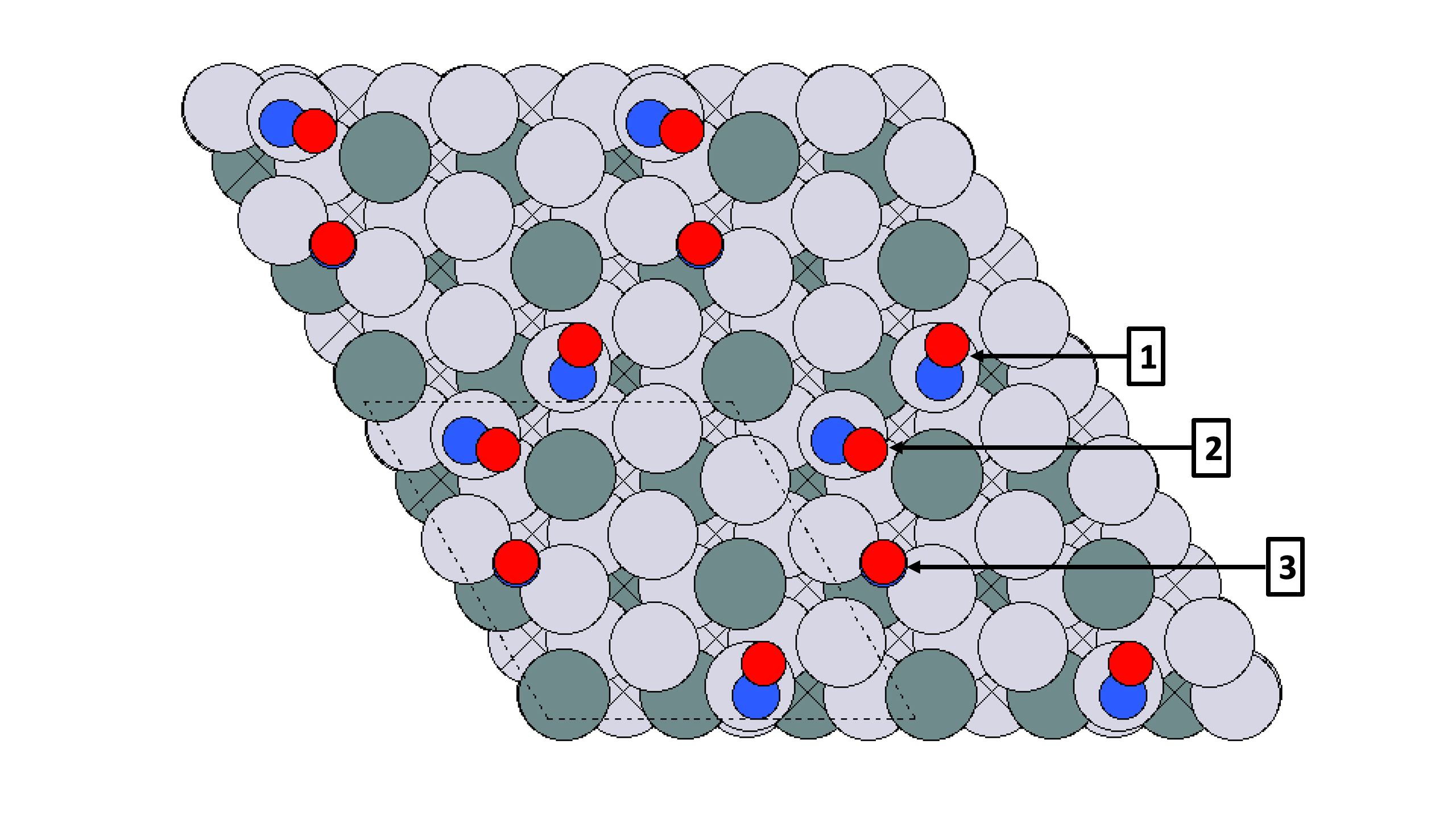
Note that in both cases, the NO are adsorbed in a bridge and two top sites. The analyze_chem_env.py can be used to find that these two cases are unique, as in first case the two NO’s are adsorbed on adjacent sites and they are on opposite sites in the second case. Further shown below are the graphs used to compare the chemical enivornment:
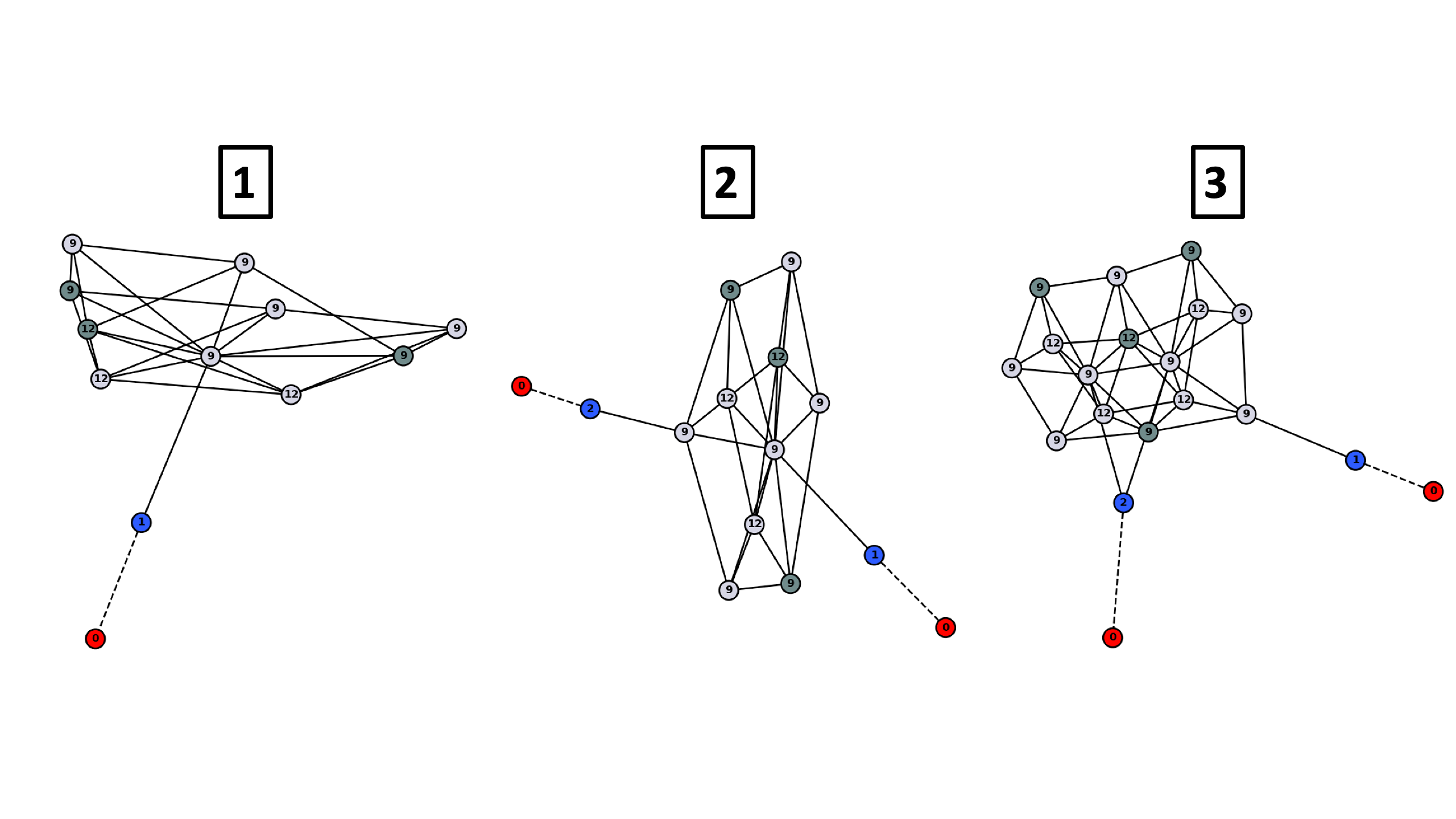
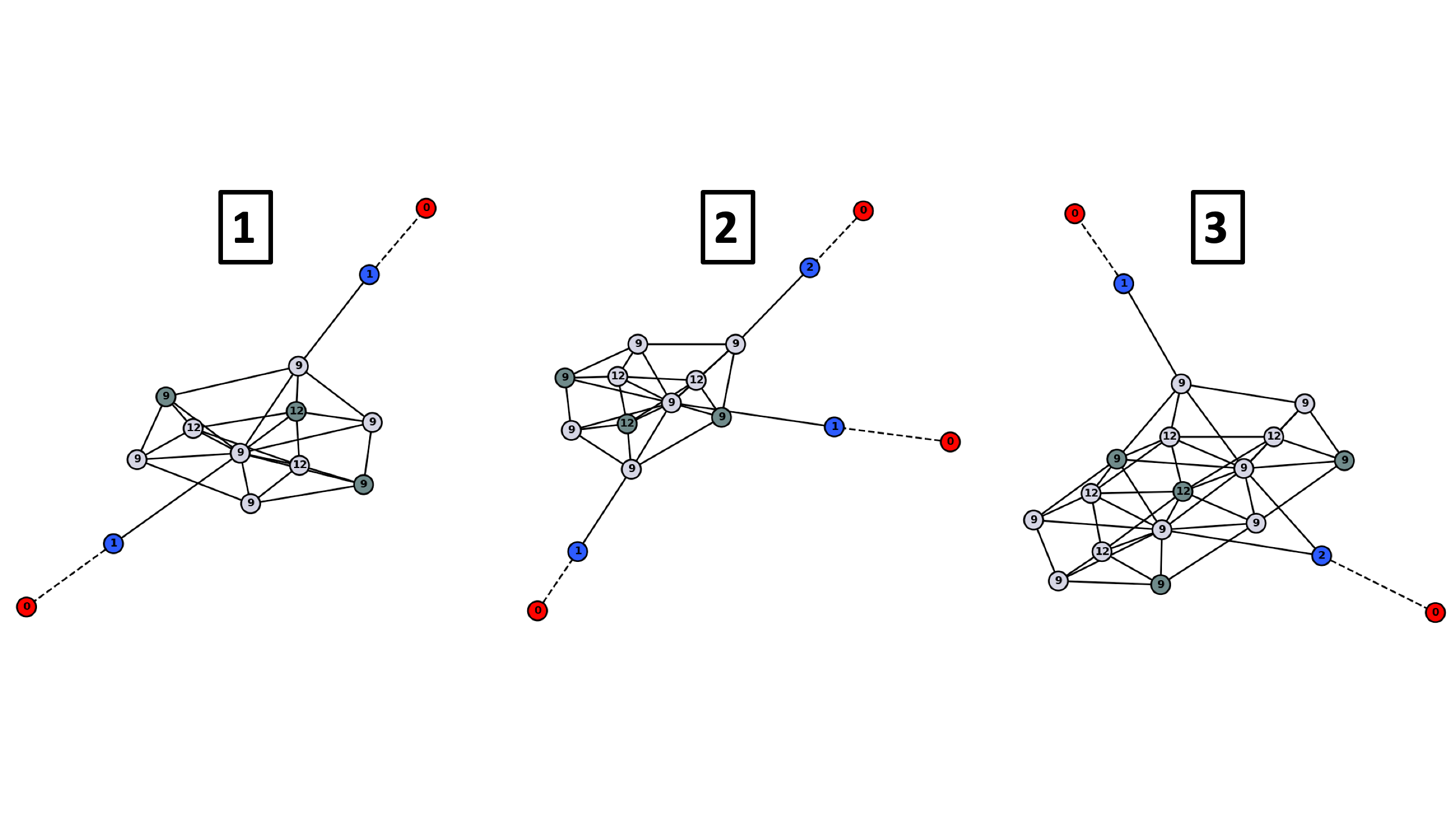
Note that in the first case, one NO molecule is isolated with no other NO adsorbed in adjacent sites. This makes the graph for this case have only 1 NO, while all the NO’s for the second case have atleast 1 NO adjacent. These kinds of graphs are compared to each other to find unique chemical environments and subsequently find unique adsorbate configurations.
generate_sites.py
This tool will find unique sites, generate normal vectors for them, then adsorb an adsorabte into that site. The adsorbate is a seperate input geometry where the adsorbate is aligned along the Z axis. The atom to bind into the site should be found at (0, 0, 0) and the adsorbate will be rotated to align with the normal of the site.
generate_sites.py --view NO.POSCAR Pt111.POSCAR
This will adsorb a NO molecule (assuming NO.POSCAR exists) into all found sites on the Pt(111) surface. This can be heavily tuned with the following settings.
- “–radius 2”: This corresponds to the graph radius for the chemical environments. This can be thought of as the number of coordination shells which should be considered. This can be tested for convergence by doing calculations on a large representative surface where one adsorbate is translated away from another and seeing how the binding energy changes. If a seperation of 3 shells is required before the energy stops changing, this is a good starting place for radius.
- “–grid ‘2,2,0’”: This corresponds to a XYZ pair for the repetitions of the cell along periodic boundaries. This has large performance penalties if raised more than needed. As long as very small cells are avoided, a value of “2,2,0” works well for 2D periodic calculations. If sites which are clearly equivalent are not based on translational symmetry, then a grid problem is likely.
- “–adsorbate-atoms ‘C,N,O,H’”: This corresponds to which atoms can be considered an adsorbate. The default assumes that adsorbates will be formed from C, O, N, and H atoms. This will have to be changed when using surfaces which contain these atoms or when using adsorbates which don’t include these atoms. More advanced ways of specifying which atoms belong to the surface can be implemented.
- “–mult 1.1”: This corresponds to the covalent radius of the atoms. In general, this can be raised if bonds are not being found that are expected or lowered if bonds are being found that are not expected. This value is a scaling factor for the covalent radius
- “–skin 0.25”: Similar to mult, this value allows for bonds to be extended by a fixed amount. This may be helpful as an additional tuning tool.
- “–min-dist 2”: This corresponds to the minimum distance allowed between adsorbates. If adsorbates would be placed closer than this, they will be rejected.
- “–no-adsorb ‘’: This corresponds to a list of elements which cannot be adsorbed to. This is helpful when prior knowledge lets you know that a specific adsorbate cannot bind to a specific element effectively.
- “–coordination ‘1,2,3’”: This corresponds to a list of coordinations which can be considered for absorption. Currently the code only works for top, bridge, and hollow sites but this will be expanded in the future.
- “–output POSCAR”: This tells the code what file extension is requested for output of files. If this is omitted, then no files will be output.
- “–output-dir .”: This tells the code what folder it should output its results into. If this is omitted, then files will be output in the current working directory.
For example, if we only wanted to adsorb molecules to the top sites of Ni atoms in a NiCu alloy, we could do the following.
generate_sites.py --output POSCAR --output-dir top-sites-Ni --coordination "1" --no-adsorb "Cu" NO.POSCAR NiCu111.POSCAR
Advanced Usage
While there is a goal of providing command line tools to perform this work, for more advanced tasks or custom properties our provided command line tools can serve as an example of how to script these tasks. The analyze_chem_env.py file serves to demonstrate the chemical_environment module and the generate_sites.py file serves to demonstrate the site_detection module. This may be useful when automation or high throughput calculations are required which can be optimized or run in parallel.